Algorithms for lattice problems in NP \(\cap\) CoNP

This site is dedicated to organizing and presenting what is known about the class of lattice problems that may have efficient algorithms. It is intended to be a living document that is updated as information comes in and as time permits.
The goal is to advance research on lattice algorithms. There are some impediments to working in this area such as its breadth, its increasingly technical nature, notational and language differences, the amount of folklore, and so on. This site provides an opportunity to have everything relevant to lattice algorithms written in one place, from one point of view, with consistent terminology, and targeted for a broader audience. Making it available to a broader audience can help build confidence that certain ranges may be difficult to solve.
Here is a picture from the paper An efficient quantum algorithm for lattice problems achieving subexponential approximation factor:
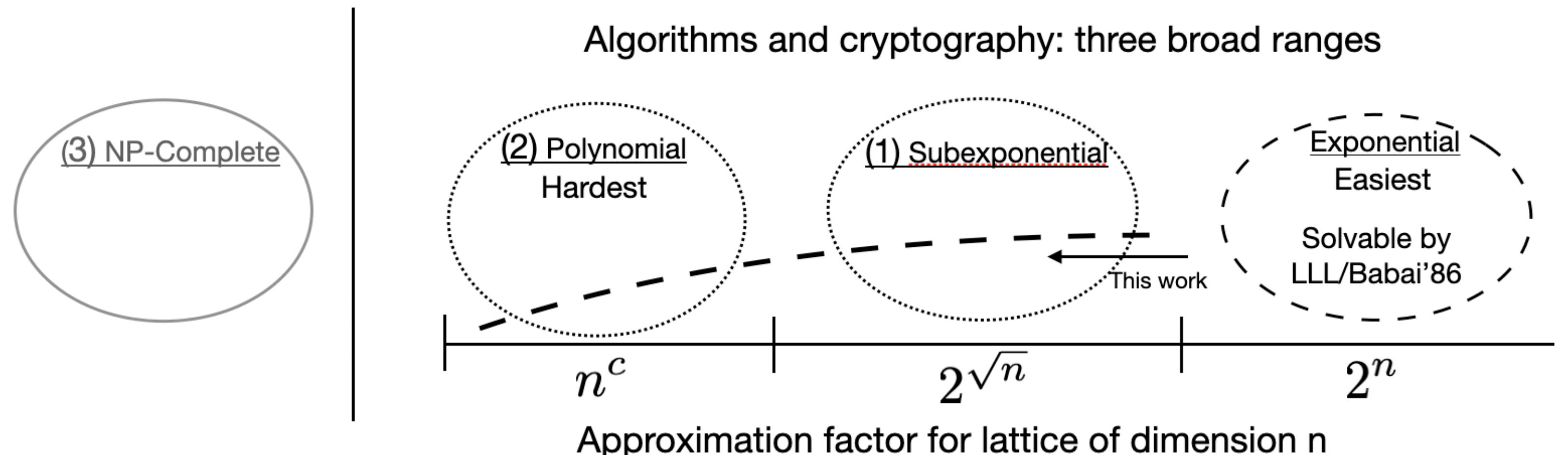
The right three regions represent NP intersect CoNP, but most work has focused on the left two regions. From an algorithms perspective, the natural approach is to push from the right side where algorithms are known. Let's do that and determine where the boundaries are.
To participate send email to latticealgorithms@gmail.com. Suggestions about all topics related to this site are welcome. This includes technical information, how to organize topics, how to visualize what is known, anything at all. Help can be public, private, or anoymous.
1. Nomenclature for this website
- Problems with efficient algorithms may be called easy, easy to solve, poly time, or polynomial time.
- Problems where no efficient algorithm are known may be called open, open problems, hard, or hard cases. These really are open problems and should not be confused with NP-hard problems which are hard in a fundamentally different way.
- \(\GapSVP\), the problem of deciding if a given lattice has a Shortest Vector Length lower or much larger than a given number, will often be called \(\GapSVL\) to better reflect the underlying problem. So \(\GapSVP=\GapSVL\) here.
- Subexponential has a few different meanings depending on the context. Here subexponential in \(n\) will typically mean a function of the form \(2^{n^\epsilon}\), for \(\epsilon <1\). An example is \(2^{\sqrt{n}}\).
- For a basis \(\pB\) of a lattice \(\pL\), basis dependent quantities like \(\|\vb_1\|\), the length of the first column of \(\pB\), will be in terms of the basis, and basis independent quantities like \(\lambda_1(\pL)\) will be in terms of the lattice. For example, if \(\vb_1\neq 0\), then the inequality \(\lambda_1(\pL) \leq \|\vb_1\|\) indicates that one quantity is basis dependent and the other is not.
- - \(n =\) dimension of an arbitrary lattice.
- \(m =\) dimension of a random lattice.
2. \(\GapSVP_\gamma\) status
\(\GapSVP_\gamma\) is the decision version of approximating the length of the shortest vector in a lattice. Given a basis \(\pB\) of an \(n\)-dimensional integer lattice \(\pL\) and a number \(d\in \R\), decide if \(\lambda_1(\pL) \leq d\) or \(d\gamma < \lambda_1(\pL)\). This the case studied in Reg09.
- As a function of the dimension \(n\):
- \(\gamma(n) = 2^{n/2}\) is poly time.
- \(\gamma(n) = 2^{n \log \log n/\log n}\) is poly time.
- The determinant of \(L\) provides information, where
- \(\gamma = 2^{\sqrt{\log \det(L)}}\) is poly time.
- The period \(\perL\) of the lattice \(\pL\) and the finite abelian group rank \(\fgr\) of \(\pL \bmod \perL\) provide information. Given a lattice \(L\), these two quantities are easy to compute. Then
- \(\gamma(n) \approx 2^{\sqrt{\fgr \log \perL}}\) is poly time.
- For example, for the class of lattices \(L\) that have \(\fgr = 1\) and \(\perL = 2^{n}\), approximation factor \(\gamma(n) \approx 2^{\sqrt{n}}\) has an efficient algorithm. Using the determinant bound for this case, the log of the determinant is at least \(\log \perL^{n-\fgr} = n^{1/2}(n-1) \approx n^{3/4} \geq \log \perL\), and the square root gives an approximation factor of \(2^{n^{3/2}}\).
- \(\fgr=1\) with an approximation factor that is a polynomial in \(n\) is an open problem.
- \(\gamma(n) \approx 2^{\sqrt{\fgr \log \perL}}\) is poly time.
2.1. Algorithm
- Given \(\pB\) for \(\pL\), compute \(\perL\), and the finite abelian group rank \(\fgr\), and change the basis to have the generators of that group.
- Run LLL on \(\pB\). Now \(\frac{\lambda_1(\pL)}{2^{\sqrt{\fgr \log \perL}}} \leq \min_i \|\vb_i^*\|\), the \(\BDD\) decoding radius, so \(\BDD\) can be solved with approximation factor \(\frac{1}{2^{\sqrt{\fgr \log \perL}}}\).
- Use the \(\GapSVL_\gamma\) to \(\BDD_{\frac{1}{\gamma}\sqrt{\frac{n}{\log n}}}\) reduction of Pei09/LM09, resulting in an approximation factor of \(\gamma(n) = 2^{\sqrt{\fgr \log \perL}} \cdot \sqrt{\frac{\log n}{n}}\) for \(\GapSVL\).
Because of the particular basis dependence algorithm, it also means that sampling from the Gaussian weighted dual lattice is possible out to some related bound.
3. Upcoming topics
- What is NP intersect CoNP (i.e., NP \(\cap\) CoNP) and why is it relevant here?
- What does it take to establish a belief that no efficient algorithm exists for a computational problem? It's not easy. For example, who has worked on it? For how long? How much expertise is necessary, and who has it? What kind of incentive is there to work on it? Are people actively discouraged from working on it for various reasons? What are the answers to these questions for factoring and LWE?
- Does the worst-to-average case reduction from lattice problems to LWE have a complexity flavor, or is it more like discrete log?
- What is the right parameter set to use for measuring progress in lattice algorithms? The dimension has long been the focus but with progress stuck for so long is that a good idea?
4. Questions
- Why does latticechallenge.org only have \(q\) = prime and not the power-of-two case? What about \(q=n^2\)?
- Which subexponential approximation factor assumptions have been made for fully-homomorphic encryption, and how do they relate to the recent algorithms?
5. Open Problems
- The driving question, way off in the distance: does a polynomial-time algorithm exist for solving any lattice problems with polynomial approximation factor?
- As a more reasonable starting point, which lattices problems can be solved for subexponential approximation factors?
- Which problems are easier to solve for special case lattices such as ideal lattices?
6. Links to lattice-based cryptography
A lot of amazing tools have been developed in lattice-based cryptography over the last couple of decades. Perhaps they can help with algorithms for lattice problems in NP \(\cap\) CoNP also. There will be some translation necessary.
7. Reductions are the tool to compare the relative computational difficulty of problems
In computer science there are not good tools to prove that efficient algorithms don't exist to solve a problem. Most problem in NP either have a polynomial-time algorithm or they can be shown to be NP-complete. NP-complete are not generally believed to have efficient classical or quantum algorithms, but they are not the topic of this site. Here the focus in on problems that are in NP$∩$CoNP. This includes the class of polynomial-time solvable problems.
A problem \(A\) reduces to a problem \(B\), written \(A \leq B\), if an algorithm for \(B\) can be used to solve problem \(A\). A reduction is an algorithm and therefore can be specified by its resources. A reduction might be computable computable \(\leq_c\), polynomial time \(\leq\), randomized \(\leq_r\), or quantum \(\leq_Q\). Reductions can be used for both algorithms and for hardness. Here \(\leq\) with no subscript will denote polynomial-time because it will be used the most.
- If \(A \leq B\) and there is a polynomial-time algorithm for \(B\), then there is a polynomial-time algorithm for \(A\) because polynomials compose.
- If \(A \leq B\) and there is no polynomial-time algorithm for \(A\), then there is no polynomial-time algorithm for \(B\).
7.1. Simple examples using polynomial-time reductions and algorithms but avoiding necessary technicality:
- Break RSA mod \(N\) \(\leq\) factor \(N\). Therefore, if there is an algorithm for factoring then there is an algorithm to break RSA.
- Solve SVP \(\leq_Q\) break LWE. Therefore, if there is no quantum algorithm for SVP, then there is no quantum algorithm for breaking LWE.
- \(\BDD \leq \SVP\) when the approximation factor is something.
8. \(\BDD\) is not \(\LWE\)
8.1. Bounded Distance Decoding (\(\BDD\)) and Learning With Errors (\(\LWE\)) are not the same problem. They are related in important ways, but they are also different in important ways.
One might say that \(\BDD \leq \LWE \leq \BDD\) to have a high-level understanding of the relationship, but what's missing in that statement are the parameters and problem definitions that give the relationships the necessary meaning.
- The theoretical connection \(\BDD \leq \LWE\) is used to conclude that an algorithm for \(\LWE\) can be used to construct a quantum algorithm for \(\BDD\).
- Concrete security involves choosing key sizes for implementations. This uses the more the direct \(\LWE\) \(\leq\) \(\BDD\) reduction, similar to Break RSA \(\leq\) Factoring. In this case a \(\BDD\) algorithm of the right parameters can be used to solve LWE, because after an \(\LWE\) instance is chosen and fixed, it is then a \(\BDD\) instance. Running \(\BDD\) algorithms on those instances is used to understand how well algorithms perform on LWE.
8.2. The classical reduction from \(\BDD\) to \(\LWE\)
The first step of the worst-case to average-case reduction in Reg09 is a classical reduction from \(\BDD\) to \(\LWE\). Here is a sketch.
Let \(\qqn\) and \(\alpha(n)\) be functions such that \(2\sqrt{n} \leq \qqn\alpha(n)\).
Let \(m(n)\) be a polynomial in \(n\).
Input: \(\pB\) for lattice \(\pL\) of dimension \(n\), target vector \(\vt = \pB\cdot \vs + \vD\), \(\|\vD\| \leq \alpha(n) \lambda_1(\pL)\).
- Repeat until \(\vs\) is computed:
- Sample \(\dv_1,\ldots, \dv_{m(n)} \in \dL\) according to a Gaussian with parameter \(\varphi_{3n}(\dL)\).
- For \(i = 1, \ldots , m(n)\):
- Compute \(\va_i = \dv_i \cdot \pB \bmod \qqn\).
- Compute \(b_i = \dv_i \cdot \vt \bmod \qqn\).
- Call the \(\LWE_{n,\qqn,\alpha}\) oracle with \((\va_1,b_1), \ldots, (\va_{m(n)}, b_{m(n)})\) and get the low-order bits the secret coefficient vector, namely \(\vs_\ell = \vs \bmod \qqn\), where \(\vs = \vs_h \qqn + \vs_\ell\).
- Set \(\vt := \frac{\vt - \pB\cdot \vs_\ell}{\qqn} = \frac{\pB\cdot(\vs_h \qqn + \vs_\ell - \vs_\ell) + \vD}{\qqn} = \frac{\pB \cdot\vs_h\qqn}{\qqn} + \frac{\vD}{\qqn}\).
Some differences between \(\BDD\) and \(\LWE\) can be seen in this reduction. The lattice given as part of the \(\BDD\) input is any lattice. The input to the \(\LWE\) problem has an associated random lattice that can be computed from the \(\va_i\)'s. The classical hardness result for \(\LWE\) uses this part of the reduction and shows that if \(\LWE\) is solvable then it is possible to approximate length of a shortest vector of an arbitrary lattice. In contrast, the length of a shortest vector in the associated \(\LWE\) lattice is easy to compute. It ends up being long, which is can be useful.
8.3. The quantum reduction from \(\varphi_0(\dL)\)-\(\SIVP\) to \(\LWE_{n,\qqn,\alpha(n)}\).
Some notation for quantum samples
To describe the steps of the quantum reduction in a somewhat concise way the notion of quantum sampling can be used to replace the classical samples. For a given distribution, a quantum sample is a quantum state whose measurement results in a sample from the same distribution.
For this reduction, let \(\Gdist{\dL,r}\) be the discrete gaussian distribution on \(\dL\) with standard deviation \(r\). This is called \(D_{\dL,r}\) in Reg09. A quantum sample of this distribution is the superposition \(\Gsup{\dL,r} = \sum_{\dv\in\dL} \sqrt{p_\dv} |\dv\>\), where \(p_\dv\) is the probability of measuring \(\dv\) from \(\Gdist{\dL,r}\). Measuring \(\Gsup{\dL,r}\) destroys the state, so the algorithm will need to create a quantum sample in each of \(m(n)\) registers, resulting in the state \(\Gsup{\dL,r}^{\otimes m(n)}\). This is tensor product notation for the state \(\Gsup{\dL,r}\Gsup{\dL,r} \cdots \Gsup{\dL,r}\), \(m(n)\) times. To summarize the notation, given the state \(\Gsup{\dL,r}^{\otimes m(n)}\), it can be measured any time to produce \(m(n)\) independent samples from \(\Gdist{\dL,r}\).
- For \(\SIVP\) the reduction will compute \(\Gsup{\dL, \varphi_0(\dL)}^{\otimes m(n)}\), where \(\varphi_0(\dL) = \frac{\sqrt{2n}}{\alpha(n)}\eta_\epsilon(\dL)\). The approximation factor is therefore not just a function of the dimension \(n\) but also of the input lattice itself. This quantum sample is enough to solve \(\SIVP\). Measuring the state will result in samples where \(n\) can be selected such that the length is at most \(\sqrt{n} \varphi_0(\dL)\).
Reduction sketch
Let \(\qqn\) and \(\pfactor(n)\) be functions.
Let \(m(n)\) be a polynomial in \(n\).
Input: \(\pB\) for lattice \(\pL\) of dimension \(n\), target vector \(\vt = \pB\cdot \vs + \vD\), \(\|\vD\| \leq \pfactor(n) \lambda_1(\pL)\)- Compute \(\Gsup{\dL,\varphi_{3n}(\dL)}^{\otimes m(n)}\).
- for \(i = 3n-1, 3n-2, \ldots, 0\):
- Measure the state \(\Gsup{\dL,\varphi_{i+1}^{}(\dL)}^{\otimes m(n)}\) to generate \(m(n)\) samples \(\dv_1, \ldots, \dv_{m(n)}\) from \(\Gdist{\dL, \varphi_{i+1}(\dL)}\).
- For \(i = 1,\ldots, m(n)\):
- Compute \(\va_i = \dv_i \cdot \pB \bmod \qqn\).
- For \(j = 1, \ldots, m(n)\):
- In new registers, compute \(\sum_{\pv \in \pL} \rho_?(\pv) \sum_{\vt} \rho_?(\vt)|\pv+\vt\>|\vt\>|0\>^{\otimes m(n)}\).
- Compute each \(b_i^{(\vt)} = \dv_i \cdot \vt \bmod 1\), giving \[\sum_{\pv \in \pL} \rho_?(\pv) \sum_{\vt} \rho_?(\vt)|\pv+\vt\> |\vt\>|b_1^{(\vt)},\ldots,b_{m(n)}^{(\vt)}\>.\]
- Compute \(\pfactor\)-\(\BDD\) using \(\LWE\) on \((\va_1, b_1^{(\vt)}), \ldots,(\va_{m(n)}, b_{m(n)}^{(\vt)})\) to erase \(\vt\), giving \[\sum_{\pv \in \pL} \rho_?(\pv) \sum_{\vt} \rho_?(\vt)|\pv+\vt\>|0\>|b_1^{(\vt)},\ldots,b_{m(n)}^{(\vt)}\>.\]
- Uncompute each \(b_i^{(\vt)}\) by computing \(\dv_i \cdot (\pv+\vt) = \dv_i \cdot \pv + \dv_i \cdot \vt \bmod 1 = b_i^{(\vt)}\), subtracting, and running backwards to get \[\sum_{\pv \in \pL} \rho_?(\pv) \sum_{\vt} \rho_?(\vt)|\pv+\vt\>|0\>|0\>^{\otimes m(n)}.\]
- Compute \(F_{q(n)}\) to get \(\Gsup{\dL,\varphi_i(\dL)}\).
- Output \(\Gsup{\dL,\varphi_0(\dL)}^{\otimes m(n)}\).

8.4.
9. Lattice parameters
9.1. Using the dimension \(n = \dim(L)\) might prevent progress.
Running times and approximation factors for lattices have typically been measured as a function of their dimension \(n\). It makes for nice, clean statements. For example, LLL is a polynomial-time algorithm to compute vectors within a \(2^n\) factor of the shortest vector. Babai's algorithm takes also takes a vector in space and computes a close lattice vector that is within a \(2^n\) factor of the closest. These approximation factors are exponential in the dimension \(n\). It can be said that there is no efficient algorithm known to achieve subexponential or polynomial approximation factors. See, for example Remark 2 and Page 8, Algorithms and Complexity. Furthermore, this has been the case for decades. There are also classes of lattice problems that are NP-hard but are not relevant here because they are not in CoNP.
The typical way to handle being stuck is to break the problem down into special cases to try to make progress. For lattices, perhaps measuring everything in terms of the dimension is preventing progress. For example, there might be an efficient algorithm for problems with a subexponential approximation factor, like \(2^\sqrt{n}\), but it's too hard to find it all at once, just like it's too hard to climb a mountain in one giant step.
As one of the L's in LLL once told me, when everyone is stuck on a problem, it is a form of art to back off the full problem and solve a subcase that is both nontrivial and solvable.
9.2. Another possibility: lattice periodicity \(\perL\) and finite group rank \(\fgrL\)
Without loss of generality, a lattice can be specified by a basis \(\matB\) and numbers \(\per_1(L),\cdots,\per_n(L)\) with the following properties. Let \(\perL\) be the minimum number such that \(\perL \Z^n \leq L\).
- For each \(i\), \(\per_i(L)\cdot \vb_i\) is a multiple of \(\perL\),
- \(1= \per_{n}(L)\ \big|\ \per_{n-1}(L)\ \big|\ \cdots\ \big|\ \per_1(L)\ \big|\ \perL\).
In particular, \(L \bmod \perL\) is a finite abelian group, and columns \(\vb_{\fgrL+1},\ldots,\vb_n\) are \(\vzero \bmod \perL\). For \(\SVP\) and \(\CVP\) those columns do not provide extra information.
10. The classical theoretical justification for LWE
Let \(q(n) = 2^{3n}\).
To understand the basis for \(\LWE_{n,n^c}\), the input to \(\GapSVL\) and \(\BDD\) includes a lattice \(L\) of dimension \(\sqrt{n}\).
| \(\LWE_{n,n^c} \leftrightarrow \LWE_{\sqrt{n},2^n}\) | As a function of the worst-case dimension \(n\), period \(q(n)\), and dimension \(m(n)\) of the associated \(\LWE\) lattice \(\rndL\), approximating the length of the shortest vector of randomly selected lattices \(\rndL\) can be done since, with high probability, \(\delta \sqrt{m(n)} \det(\rndL)^{1/n} \leq \lambda_1(\rndL) \leq \sqrt{m(n)}\det(\rndL)^{1/n} = \sqrt{m(n)}q(n)^{1-n/m(n)}\) for a constant \(\delta\). |
| \(\Bigg\uparrow\) | |
| \(\BDD\) dimension \(\sqrt{n}\) | |
| \(\Bigg\uparrow \quad i.e., \GapSVL \leq \BDD\) | |
| \(\GapSVL\) dimension \(\sqrt{n}\) | Approximate the length of shortest vector a lattice \(L\) that is taken from a certain subset of \(n\)-dimensional lattices. |

Notes:
- \(\GapSVL\) is known as \(\GapSVP\) in the literature. Here the name is changed for two reasons. First is that it has a mnemonic meaning: the Shortest Vector Length. Second, when referring to the problem as \(\GapSVP\), it is easy to miss the fact that \(\LWE\) is based on computing the length of a shortest vector, which may be much easier than computing a shortest vector.
- \(\BDD \leq \LWE_{2^{3n}}\) is a special case in Reg09. It is used as a black box in Pei09.
- \(\GapSVL \leq \BDD\) is from Pei09.
11. Ideas that may or may not work
- Amplitude amplification on a state containing shapes around each lattice point.
- Partition lattices in various ways to make progress.
12. Road blocks
12.1. Cannot do the following
- Using FHE, given \(\matA, \matA\vs+\ve\), compute \(\matA', \matA'(q/2)\vs+\ve'\).
12.2. Besides not finding an algorithm yet, are there other ways to describe why the various problems might or might not have an efficient algorithm?
13. Some lattice facts to organize
13.1. Lattices and their duals
13.1.1. Lattices come in pairs \((L,L^*)\)
- \(1 \leq \lambda_1(L) \cdot \lambda_n(L^*) \leq n\).
- \(\eta_{\eps(n)}(L) \leq \frac{\sqrt{n}}{\lambda_1(L^*)}\), for \(\eps(n) = \frac{1}{2^n}\).
- \(c\frac{\lambda_n(L)}{n} \leq c \frac{1}{\lambda_1(L^*)} \leq \eta_{\eps(n)}(L)\) for \(\eps(n) = o(1)\) and any constant \(c\).
- For \(\vw = \va\matB^{-1} \in L^*, \vv = \matB \vc \in L\), \(\vw \cdot \vv = \va \cdot \vc\).
13.1.2. Dual problems, approximation factors
- \(\SVP\) vs. \(\CVP\)
- \(\GapSVL\) vs. \(\GapCVP\)
13.2. Other
13.2.1. \(\forall\) bases \(\matB\) of \(L\):
- \(\minGS \leq \lambda_1(L)\).
- \(\det(L) := \vol(\calP(\matB)) = \prod_i \|\vb_i^*\|\).
- \(\det(L) \leq \prod_i \|\vb_i\|\).
- \(\det(L) = \sqrt{\det(\matB^t\matB)}\), and for the full-rank case, \(\det(L) = |\!\det(\matB)|\).